Understand Transformer Paper Through Implementation

a detailed implementation of binary classification using transformer encoder

Introduction

In the recent years, transformer architecture has gain much popularity in sequence modelling replacing the previously state of the art deep learning model such as LSTM and GRU, transformer also show capability in both NLP and computer vision which is very interesting, it open the gate of possibilities to build a neural network model that works well across multiple domains. In this article we will implement a binary classification model IMDB dataset , which is a large movie review dataset contain labeled review as positive or negative.

Self Attention

Attention is a neural network layer that map sequence to sequence set to set. There are two kind of attention layer, self attention and cross attention, each can be a hard attention or soft attention. Suppose that $\{x_i\}_{i=0}^t$ a set of row vectors where $x_i^{\mathsf{T}}\in \mathbb{R}^d$, if $\{x_i\}_{i=0}^t$ is an input of self attention then the output is a set of linear combination $h=\alpha_0x_0+\dots +\alpha_tx_t=aX$, where $a={\begin{bmatrix} \alpha_1 & \alpha_2 & \dots & \alpha_t\\ \end{bmatrix}}^{\mathsf{T}}$ is a row vector called attention vector. When $a$ is one hot encoding then the layer is called hard attention, otherwise it is called soft attention and the total sum of elements in $a$ equals to $1$, in practice we represent attention vectors as matrix $A$, which each row of $A$ is attention vector. In this article to match the mathematical convention with the original transformer paper we will represent sequence of vectors as matrix where the vertical axis is the sequence length and the horizontal axis is the vector dimension as depicted in the following diagram.

The sequential order of attention layer input might lost during the computation, for instance let $V \in \mathbb{R}^{4\times3}$ , is a matrix represent sequence of four 3-dimensional (row) vectors, attention layer multiplies $V$ with an attention matrix $A$, if $A$ happened to be a permutation matrix we might lose the order information of $A$, to understand this please take a look at following illustration:

as you can see that $A$ permutes the rows of matrix $V$ which mean it permutes the sequence order, in other words attention ignore positional information, so attention maps set to set, however the transformer paper propose a method to enforce attention to map sequence to sequence by encode a positional information and inject it to input matrix which will be explained in the later section of this article.

Queries, Keys and Values

Transformer’s attention layer was inspired by key-value store mechanism, we usually find such mechanism in something like programming language data structure, for example python built-in dictionary, python dictionary has key-value pairs from which we can fetch a value by feeding a query to the dictionary, the dictionary then compare the query to each key if the query match a key it will return the value corresponding to that key, to mimic this behaviour, transformer’s attention layer transform input matrix $X$ into three entities; query, key, and value analogous to python dictionary. These entities are generated by transforming each row vector of input matrix with linear transformation, for instance to get a value vector $v$, multiply a row vector $x$ of $X$ with a matrix $W_{value} \in \mathbb{R}^{\text{input dimension}\times d_v}$, the same rule applies for key and query vector $$v=xW_{value}$$ $$k = xW_{key}$$ $$q=xW_{query}$$ It is easy to show above operation in matrix form as follow $$V=XW_{value}$$ $$K=XW_{key}$$ $$Q=XW_{query}$$ Lets get some intuition about this concept, suppose that $q$ is a query vector (a row of $Q$ matrix), $i^{th}$ element of attention vector $A$ is similarity value between the $q$ and the $i^{th}$ element of key matrix denoted by $k_i$, there are many ways to measure similarity between two vectors, one of the simplest form of similarity measure is dot product between $q$ and $k_i$, to compute dot product for each key vectors we can compute $qK^{\mathsf{T}}$ this mean we compute a query with every row of key matrix, furthermore to compute similarity between all query vector and all key vectors, simply calculate $QK^{\mathsf{T}}$.

As mentioned in the previous section each attention vector (row of attention matrix $A$) should sum to 1 as in probability distribution, to achieve this we can apply $\text{argsoftmax}(\cdot)$ in the element-wise manner for each row of $A$ as follow $A=\text{argsoftmax}(\frac{QK^{\mathsf{T}}}{\beta})$ where $\beta$ is normalizing factor, the scaling factor is needed to make the variance stable as explained in the next section, to make $A$ hard attention we can replace $\text{argsoftmax}(\cdot)$ with $\text{argmax}(\cdot)$. Then output of self attention is $H=AV$ a row of $H$ is $h=aV$ without losing generality let imagine that $a$ is a one hot encoding vector intuitively multiplying vector $a$ with matrix $V$ is choosing a row of $V$ then return it as $h$, when $a$ is not a one hot encoding it will “mix” some rows of $V$ then return it as $h$. The case where $a$ is a one hot encoding is almost identical with python dictionary meanwhile the softattention case is more like the flexible version of python dictionary, to better understand this let make an example, given a python dictionary : H = {’a’:’cat’,’b’:’dog’,’c’:’dragon’} suppose that we feed ‘b’ as query to the dictionary, in other word we are asking to the dictionary about what is the *value* corresponding to ‘b’ key, the dictionary then compare the query to each keys if there is a match it will return the value corresponding to the matched *key*, this is analogy with computing $a=qK^{\mathsf{T}}$ each element of $a$, $\alpha_i$ represent similarity between $k_i$ and $q_i$ where $q$ is a row vector of matrix $Q$. fetching value of H[’b’] is analogous to computing $h = aV$. The only difference here is that in attention query and key does not to be exactly the same in order to be match, this rule does not apply for python dictionary though. let’s make an example and a visualize the matrix shape to enhance our understanding, suppose that our input $X$ is a 4 sequence of 3-dimensional row vector, and $d_k=d_v=d_q=2$ are dimension of key vectors, value vectors and query vector respectively and $W_k\in\mathbb{R}^{3\times d_k},W_v\in\mathbb{R}^{3\times d_v}, W_q\in\mathbb{R}^{3\times d_q}$ are matrix that will transform $X$ to key, value and query matrix.

to summarize this section the attention layer can be easily visualize through the following diagram

or in more compact diagram, attention layer will look like the following diagram

Scaled Argsoftmax

This section mostly will deal with the mathematical derivation of the scale factor of scaled argsoftmax which the original paper does not explain in detail, if you are already familiar with probability theory for specific with notions of variance and mean of a random variable then this section is safe to be skipped.

Large value of key vectors dimension ($d_k$) will cause high variance in $QK^{\mathsf{T}}$ which will cause a negative impact on training as the paper mentioned :

We suspect that for large values of $d_k$, the dot products grow large in magnitude, pushing the softmax function into regions where it has extremely small gradients. To counteract this effect, we scale the dot products by $\frac{1}{\sqrt{d_k}}$

However it is unclear why the scaler should be $\frac{1}{\sqrt{d_k}}$, original paper mention that the reason is:

To illustrate why the dot products get large, assume that the components of $q$ and $k$ are independent random variables with mean 0 and variance 1. Then their dot product, $q \cdot k = \sum^{d_k} _{i=1}q_ik_i$, has mean 0 and variance $d_k$

The first time I read above phrase, it was not very obvious for me, why the variance of $q\cdot k$ is $d_k$ and also why the scaler is $\frac{1}{\sqrt{d_k}}$. In this section we will proof it mathematically

The original paper of transformer assumes that the readers have some degree of familiarity with basic probability theory, but if you are like me, not super familiar with probability theory here is some refresher. suppose that $X$and $Y$ are both identical and independent random variable, then derived directly from variance definition it is easy to show that

Then $\begin{aligned}{\text{Var}[XY]} &= E[X^2Y^2]-E[XY]^2 \\ &= {\color{orange}E[X^2]}{\color{teal}E[Y^2]}-E[X]^2E[Y]^2\\&=({\color{orange}\text{Var}[X]+E[X]^2})({\color{teal}\text{Var}[Y]+E[Y]^2})-E[X]^2E[Y]^2 \\&=\text{Var}[X]\text{Var}[Y]+\text{Var}[X]E[Y]^2+\text{Var}[Y]E[X]^2+{\color{purple}E[X]^2E[Y]^2-E[X]^2E[Y]^2}\\&=\text{Var}[X]\text{Var}[Y]+\text{Var}[X]E[Y]^2+\text{Var}[Y]E[X]^2\end{aligned}$ Let assume that each row vector of $K$ and $Q$ has zero mean and unit variance. Suppose that $k,q$ is column vector of $K$ and $Q$ respectively then $k\cdot q$ is an element of $K^{\mathsf{T}}Q$ and let consider. $\begin{aligned}\text{Var}[k\cdot q]&= \text{Var}[\sum _{i=1}^{d_k}k_iq_i]\\&=\sum _{i=1}^{d_k}\text{Var}[k_iq_i]\\&=\sum _{i=1}^{d_k}\text{Var}[k_i]\text{Var}[q_i]+{\color{teal}\text{Var}[k_i]E[q_i]^2}+{\color{orange}\text{Var}[q_i]E[k_i]^2}\\&=\sum _{i=1}^{d_k}1+{\color{teal}0}+{\color{orange}0}\\&=d_k\end{aligned}$ Now elements of $QK^{\mathsf{T}}$ has zero mean and $d_k$ variance, the variance depend on the dimension of the key or query vector, this is unwanted behaviour since changing the dimension will also changing it’s variance too low variance will cause the argsoftmax output to be hard and vice-versa. We want to keep zero mean and unit variance, since $\text{Var}(\alpha X)=\alpha^2\text{Var(X)}$ then we should scale $QK^{\mathsf{T}}$ by $\sqrt d_k$ such that $\begin{aligned}\text{Var}[\frac{k\cdot q}{\sqrt d_k}]&=(\frac{1}{\sqrt d_k})^2Var[k\cdot q]\\&=\frac{d_k}{d_k}\\ &= 1\end{aligned}$

hence the attention matrix become $A=\text{argsoftmax}(\frac{K^{\mathsf{T}}Q}{\sqrt d_k})$

Positional Encoding

Remember in the previous section the input of attention layer might lost it’s sequential order information. Before diving into the method proposed by author to enforce attention layer to maintain its input posititional information, lets think of some possibilities that we could do to maintain the positional information of attention layer input.

1. The naive solution is concatenating index to the input for instance ${[0,v_1], [1,v_2], … ,[n,v_n]}$ this could work but this has serious drawback when we normalize it the index value will be varied depending on the sequence length.
2. Use binary number as index instead of decimal, this approach seem promising but still has flaw since the euclidean distance between two adjacent index is not consistent

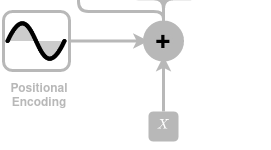
The authors of paper attention is all you need propose a method using the following function $\text{PE} (pos,2i) = \sin\left({\frac{pos}{1000^{\frac{2i}{\text{d\_model}}}}}\right)$ $\text{PE} (pos,2i+1) = \cos\left({\frac{pos}{1000^{\frac{2i}{\text{d\_model}}}}}\right)$ this function is choose because it has desired mathematical properties, $PE(pos,2k+i)$ is a linear mapping from $PE(pos, 2k)$, so the distance between index is consistent, and also the embedding is not concatenated with the input instead it use element-wise addition, the author argument that empirically there is no much different between concatenating and element wise addition between positional encoding with the input and pointwise addition yield small memory footprint. In recent development there are other ways to inject positional information to transformer input, but it is out of scope of this article.

Multi Head Attention

Multihead attention layer is simply multiple copies of attention layer where each copy does not share it’s weight parameters, on the top of it we add concatenation and fully connected layer to merge back the shape to the original single head output shape

Build a Classifier Based on Transformer Architecture

Now we have nuts and bolts needed to build our transformer architecture, time to put them together. In the original paper transformer consist of two parts encoder and decoder, but in this article we will not implement the decoder part, lets left it for next article, instead we will build the encoder part only of the transformer then add classification head on the top of it

as you can see from the diagram, we have skip connection or residual connection like the one that resnet has, its connect the pointwise addition positional encoding to add norm layer, add norm layer simply matrix addition and layer normalization.

Detailed Implementation

In this article we will not implement the sequence to sequence transformer like the one that demonstrated in the paper rather we will implement the simpler one; classification transformer that classify if a sentence has positive or negative sentiment on IMDB dataset. Implementing the sequence to sequence transformer like in the original paper need more effort since it also need us to implement beam search, I think i will try it in the next article

Generate Key, Query, Value Matrices

The first thing we should do is to generate Key, Query and Value matrix this can easily achieved by using torch.nn.linear(input_dim,head_size*d_model) , we want the query tensor has [batch_size, sequence_length, head_size*d_q] the same size apply to key, and value vectors.

Split Head

Remember that our query from previous operation has the shape [batch_size, sequence_length, head_size*d_q] . For simplicity let assume we have batch_size = 1 so if we by squeezing the batch dimension we have [sequence_length, head_size*d_q] what we going to do is to view the tensor to be [sequence_length, head_size, d_q] simply illustrated in the diagram below

why we should split the head? it is because we will compute softargmax along the horizontal axis to make the horizontal axis sum to 1, if we don’t split we will end up applying softargmax across all head,next what we want to achieve is to make attention vector to sum up to one for each single head. This operation can be done by using .view(batch_size, sequence_length, self.head_size,d_model) function from pytorch, but we are not done yet, we will compute matrix multipication between $Q$ and $K^{\mathsf{T}}$ for each batch and each head, we will use pytorch’s `@` operator but we should make the sequence_length and d_model axis to the right side, since the attention matrix size is [sequence_lengh, d_model] so we want make each tensor $Q,K,V$ to be has this shape [batch_size,head_size, sequence_length, d_q or d_k or d_q respectively] to do that we switch axis 1 and axis 2 using transpose(1,2) . The overall code now should be like this:

import torch import torch.nn as nn class MultiHeadAttention(torch.nn.Module): def __init__(self,input_dim, head_size,d_model): super(MultiHeadAttention, self).__init__() d_q, d_k, d_v = d_model self.head_size = head_size self.W_q = torch.nn.linear(input_dim,head_size*d_q) self.W_k = torch.nn.linear(input_dim,head_size*d_k) self.W_v = torch.nn.linear(input_dim,head_size*d_v) def split(self,X): batch_size, sequence_length, num_head_times_d_model = X.size() d_model = num_head_times_d_model//self.head_size X = X.view(batch_size, sequence_length, self.head_size,d_model).transpose(1,2) return X def forward(self,X_query,X_key,X_value): Q,K,V = self.W_q(X_query), self.W_k(X_key), self.W_v(X_value) Q,K,V = self.split(Q), self.split(K), self.split(V)

Scaled Dot Product Attention

Implementing scaled dot product is pretty straight forward, but one thing should be noticed since the first and second axis of the key tensor is batch size and head size respectively, then the transpose should be done in third axis and fourth axis so it become K_T = K.transpose(2,3) the rest of scaled dot product should look like this

Now let update our multihead attention network and add scaled dot product to it dont forget to concat the result from [batch_size,head_size, sequence_length, d_model] to [batch_size sequence_length, d_model*head_size] simply by reversing the previous process of splitting the head X = X.transpose(1,2).contiguous().view(batch_size, sequence_length, self.head_size*d_model). Okay now this is the complete code of multihead attention

Feed Forward Network

This is a simple two layer multilayer perceptron with with ReLU activation in the middle which the input and output has size of d_model

Positional Encoding

The size of the positional encoding will be [max_len, d_model] and for numerical stability we modify denominator to be $\exp(\log(10000.0)\frac{2i}{\text{d\_model}})$ instead of using the original equation

import torch import torch.nn as nn class PositionalEncoding(nn.Module): def __init__(self, d_model, max_len, dropout_prob): super(PositionalEncoding, self).__init__() self.dropout = nn.Dropout(p=dropout_prob) position = torch.arange(0, max_len) position = position.float().unsqueeze(dim=1) pe = torch.zeros(max_len, d_model) div_term = torch.exp(torch.arange(0, d_model, step=2) * (-math.log(10000.0) / d_model)) pe[:, 0::2] = torch.sin(position*div_term) pe[:, 1::2] = torch.cos(position*div_term) self.register_buffer('pe', pe) def forward(self, x): batch_size, seq_len, d_model = x.size() return self.dropout(self.pe[:seq_len, :].unsqueeze(0)+x)

Encoder

Lets take a look at the encoder architecture from the original diagram from the author, we need multihead attention, positional encoding, layer normalization, and mlp.

Word Embedding

Now lets implement the part that add positional encoding to the vector encoding as subclass of torch.nn.Module for specific we are implementing this part

Encoder

Transformer Classifier

We will add simple linear layer on the top of transformer for classification, I will not put the entire code here the other part which is training loop and dataset loading was taken from Alferdo Canziani great lecture. You can to access my complete code

class TransformerClassifier(nn.Module): def __init__(self, num_layers, d_model, head_size, conv_hidden_dim, input_vocab_size, num_answers): super().__init__() self.encoder = Encoder(num_layers, d_model, head_size, conv_hidden_dim, input_vocab_size, maximum_position_encoding=10000) self.linear_classifier = nn.Linear(d_model, num_answers) def forward(self, x): x = self.encoder(x) x, _ = torch.max(x, dim=1) x = self.linear_classifier(x) return x

Conclusion

Implementing transformer is not trivial matter even when the authors say that idea behind transformer is simple but technical detail make the difficulty exponentially increasing.