Generative Adversarial Network with Bells and Whistle

Dissecting GAN paper and it's implementation

Overview

This section will explain the general idea about GAN (Generative Adverserial Network). Broadly speaking from probabilistic perspective there are two kind of mathematical models; generative model and discriminative model, GAN as it's name suggest falls into the first cathegory, so here we will focus on generative model. To make things easier to understand let's make an analogy, let say I have data in the form of images for specific the data is a collection of some of Pablo Picasso paintings, the generative model is a model that approximate the probability distribution that generate the paintings, such that the model able generate a new paintings that look like Pablo Picasso painting, but have not seen before. Each pixel data (normalized so that the values are between 0 and 1) in the paintings can be represented as vector of probabilities that is generated by $\mathbb{P}_{data}$ which is an unknown probability distribution and we wish to approximate it.

We will approximate $\mathbb{P}_{data}$ with a parametric function $G(z,\theta_g)$ which is a function of random variable $Z \sim \mathbb{P}_z$ and has distribution $\mathbb{P}_{g}$. The authors of GAN call $G(z,\theta_g)$ as generator and the function is in the form of artificial neural network. There are many ways to make generator generates sample as close as possible to samples that are generated by $\mathbb{P}_{data}$ for instance we can set a loss function between our generator's samples and real data then minimize the loss function with somekind of optimization algortihm, this is kind of method is a direct approach to the problem, instead of using direct approach GAN framework is inspired by min-max game from game theory, by introducing a new function called discriminator $D(x)$ with distribution $\mathbb{P}_{\text{is real}}$. Discriminator inputs are samples from $\mathbb{P}_{data}$ and $\mathbb{P}_{g}$ and return the probability of input was generated by $\mathbb{P}_{data}$, so the perfect discrimiator will return 1.0 if the input comes from real data and return 0.0 if input comes from generator, we can also consider discriminator as an "ordinary binary classifier" which classify wheter a data is real or fake. On the other hand generator tries to generate samples to look as close as possible to real data in order to outsmart the discriminator or in other word it try to make discriminator to classify an input as real whenever the input is fake (generated by generator). More formally discriminator and generator aims are as follow:

Discriminator Task:

• Maximize the value of $\mathbb{P}_\text{is real}(x_1,x_2,\dots,x_n)$ where $x_1,x_2,\dots,x_n$ are samples from real dataset
• Minimize the value of $\mathbb{P}_\text{is real}(G(z_1),G(z_2),\dots,G(z_n))$ where $G(z_1),G(z_2),\dots,G(z_n)$ are samples generated by generator

Generator Task:

• Maximize the value of $\mathbb{P}_\text{is real}(G(z_1),G(z_2),\dots,G(z_n))$

From the list above we can see that generator and discriminator competing to each other, this raise some important questions, for instance how come this form of competing model achieve our main goal a.k.a make a model that can generate samples that look like real data. When we suppose to stop the training ?. To answer those questions we will start by defining how our criterion should look like.

Setting up the Criterion

Let's begin with the first task of discriminator, Suppose that $x_1,x_2,\dots,x_n$ is our real samples we wish to maximize $\mathbb{P}_\text{is real}(x_1,x_2,\dots,x_n)=\prod_{1}^{n}\mathbb{P}_\text{is real}(x_i)=\prod_{1}^{n} D(x_i)$, but from computation point of view choosing this value as criterion is a bad decision since it saturate small probability value to zero, here is a code snippet that illustrate the phenomena

From the output of the code above, we can see that small values equal to zero after multipication, which is obviously not the exact value, this is caused by the decimal rounding computer does, and since we multiply many smalls values that are rounded down the result become extremely small as the result it close to zero then computer round it to zero, as an alternative since logarithm function is strictly increasing function hence $\log\left[\prod_{1}^{n} D(x_i)\right]=\sum_{1}^{n} \log D(x_i)$ will serve the same purpose, since it is only the scaled version of $\prod_{1}^{n} D(x_i)$. In statistics it is usually called log-likelihood, and since the dataset can be considered as generated by empirical distribution, we can express the log-likelihood in term of expectation,

With the same line of reasoning for the second task of discriminator we want to maximize the value of $n\mathbb{E}_{z\sim \mathbb{P}_g}\left[1-log(D(G(z)))\right]$, note here we turn minimizing task into maximizing task, so to do both task we with to maximize

Since $n$ is only a scaler we can drop $n$ such that we want to maximize

Now move to the goal of generator, if we denote optimal discriminator as $D^* = \text{argmax}_D V(G,D)$ then the goal of generator is to minimize

Optimal Discriminator

In this section we aim to find $D^{*}(x)= \text{argmax}_{D}V(D,G)$. By the Law of Unconcious Statistician we get this equation

hence

Now we want to find the value of that maximize the integran by using elementary calculus,i.e setup the derivation to zero, as follow:

So we get the optimal value for discriminator i.e $D^{*}(x)=\frac{\mathbb{P}_{data}(x)}{\mathbb{P}_g(x)+\mathbb{P}_{data}(x)}$

Optimal Generator

Now we have an optimal discriminator, next we want to find $G^* = \text{argmax}_G V(G,D^{*})$ but let's first expand $V(G,D^{*})$ :

So here we have nice interpretation because it is easy to find the minimium now, the minimum value of Jensen-Shanon divergence is atained when $\mathbb{P}_{data}(x)=\mathbb{P}_g(x)$ which cause $D^{*}(x)=\frac{\mathbb{P}_{data}(x)}{\mathbb{P}_g(x)+\mathbb{P}_{data}(x)}=\frac{1}{2}$ in other words when the min-max game equilibrium between generator and discriminator achieved, discriminator always return 0.5 for both fake and real data, which mean the discriminator is confused and cannot tell the difference between real and fake data. So theoritically the best time to stop the training is when discriminator return 50% confidence for both samples that generated by generator or real data, but this is only half of the story, we cannot guarantee that our neural network model or our optimization algortihm can achieve that condition.

Training GAN

Training GAN is somekind of art as it is not as straight forward as training "conventional" neural network architecture. The original paper of GAN itself does not provide detail about training procedure but more like general framework and the detail is left to us. Since GAN is very popular many researchers and engineers working on it, there is some nice article out there the provide technique to train GAN effectively such as ganhack ganhack, although ganhack is quite outdated but we will use some tips from them to train our GAN implementation here.

Training Discriminator

Remember that our discriminator goal is to maximize $\mathbb{E}_{x\sim \mathbb{P}_{data}}\left[\log(D(x))\right]+\mathbb{E}_{z\sim \mathbb{P}_z}\left[\log(1-D(G(z)))\right]$ notice that we can turn is maximizing problem into minimizing binary cross entropy loss and the sthocastic version (sum over batch) will look like this $L_{\text{BCE}}=-\sum^{n}_{i=1}y_i\log{\hat{y}_i}+(1-y_i)\log(1-\hat{y}_i)$ according to ganhack tips it is better to split the batch between real batch and fake batch. Feed forward the fake-only batch compute the loss, feed forward the real-only batch compute the loss, sum up both loss from real-only and fake-only batch then compute the gradient, finally update weight. As for illustration below is diagram of discrimiator forward and backward propagation. The blue line is the flow of forward propagation from real data to summing operator, and the yellow is from fake data, the red line is the flow of gradients from summed loss to discriminator.

Training Generator

Training generator is straight forward since we will only feed noise. The quirk is only we will not minimize $\mathbb{E}_{z\sim \mathbb{P}_z}\left[\log(1-D(G(z)))\right]$ rather than maximize $\mathbb{E}_{x\sim \mathbb{P}_{data}}\left[\log(D(G(z)))\right]$ hence we should assign 1.0 as label (true label) for generator output during training the generator

GAN inference

The inference is very straigh forward, just ignore the discrimiator part, generate noise and feed it to generator

Implementation

The code implementation is in python I have tried to make the code as readable as possible by minimizing the boilerplates, we will use pytorch framework to help with the automatic differentiation part for backpropagation which is not essential in this article, also the neural network model for discrimiator and generator are mlp with super simple architecture, and the BCE loss is written explicitly to enhance understanding, but in practice I really recommend to use nn.BCELoss() from PyTorch since it is well optimized and battle tested.

Import needed library, and use manual seed so we will get the same result if we run it several times from __future__ import print_function #%matplotlib inline import torch import torch.nn as nn import torch.optim as optim from torchvision import transforms from torchvision.datasets import MNIST from torch.utils.data import DataLoader import imageio import random import matplotlib.pyplot as plt import numpy as np # Set random seed for reproducibility manualSeed = 999 random.seed(manualSeed) torch.manual_seed(manualSeed)

We will use MNIST dataset, for ease of use let use the one provided by pytorch transform = transforms.Compose([ transforms.ToTensor(), transforms.Normalize((0.5,),(0.5,)) ]) to_image = transforms.ToPILImage() trainset = MNIST(root='./data/', train=True, download=True, transform=transform) trainloader = DataLoader(trainset, batch_size=100, shuffle=True) device = 'cuda'

Now define our simple generator and discrimiator architecture class Generator(nn.Module): def __init__(self): super(Generator, self).__init__() self.n_features = 128 self.n_out = 784 self.mlp = nn.Sequential( nn.Linear(self.n_features, 256), nn.LeakyReLU(0.2), nn.Linear(256, 512), nn.LeakyReLU(0.2), nn.Linear(512, 1024), nn.LeakyReLU(0.2), nn.Linear(1024, self.n_out), nn.Tanh()) def forward(self, x): x = self.mlp(x) x = x.view(-1, 1, 28, 28) return x class Discriminator(nn.Module): def __init__(self): super(Discriminator, self).__init__() self.n_in = 784 self.n_out = 1 self.mlp = nn.Sequential( nn.Linear(self.n_in, 1024), nn.LeakyReLU(0.2), nn.Dropout(0.3), nn.Linear(1024, 512), nn.LeakyReLU(0.2), nn.Dropout(0.3), nn.Linear(512, 256), nn.LeakyReLU(0.2), nn.Dropout(0.3), nn.Linear(256, self.n_out), nn.Sigmoid()) def forward(self, x): x = x.view(-1, 784) x = self.mlp(x) return x

Define our hyperparameter num_epochs = 50 lr = 0.0002 beta1 = 0.5 ngpu = 1 latent_variable_dim =128

Define loss function and optimizer, here in practice it is possible that discrimiator return zero and log at zero is undefined, to fix this we will add very small number epsilon = 1e-10 , to the output of discriminator def binary_cross_entropy(pred, y): epsilon = 1e-10 return -((pred+epsilon).log()*y + (1-y)*(1-pred+epsilon).log()).mean() generator_model = Generator().to(device) discriminator_model = Discriminator().to(device) # Establish convention for real and fake labels during training real_label = 1. fake_label = 0. discriminator_optimizer = optim.Adam(discriminator_model.parameters(), lr=lr, betas=(beta1, 0.999)) generator_optimizer = optim.Adam(generator_model.parameters(), lr=lr, betas=(beta1, 0.999))

Write function for viewing the generated results def view_result(generator_net, batch = 8): # Create batch of latent vectors that we will use to visualize noise = torch.randn((batch,128), device=device) with torch.no_grad(): output = generator_net(noise) #re-arange [NxCxHxW] to [NxHxW] since channel is 1 we will squeeze it output = output.permute(1,0,2,3).squeeze() output_np = output.cpu().detach().numpy() output_np = np.hstack(output_np) print(output_np.shape) plt.imshow(output_np)

Train our GAN and wait for some minutes img_list = [] G_losses = [] D_losses = [] iters = 0 print("Starting Training Loop...") # For each epoch for epoch in range(num_epochs): # For each batch in the dataloader for i, data in enumerate(trainloader, 0): # ------------------------------------------------------------------# # Update Discriminator model: maximize log(D(x)) + log(1 - D(G(z))) # # ------------------------------------------------------------------# # Train with batch from real data discriminator_model.zero_grad() real_cpu = data[0].to(device) b_size = real_cpu.size(0) label = torch.full((b_size,), real_label, dtype=torch.float, device=device) # Forward real data batch through D output = discriminator_model(real_cpu).view(-1) # Calculate loss binary cross entropy for real batch errD_real = binary_cross_entropy(output, label) # Calculate discriminator gradient errD_real.backward() D_x = output.mean().item() ## Train with samples generated by generator # Generate batch of latent vectors noise = torch.randn((b_size,128), device=device) # Generate batch of fake images using generator fake = generator_model(noise) label.fill_(fake_label) # Classify all fake images batch with discriminator output = discriminator_model(fake.detach()).view(-1) # Calculate D's loss on the all fake images batch errD_fake = binary_cross_entropy(output, label) # Calculate the gradients for this batch, accumulated (summed) with previous gradients errD_fake.backward() D_G_z1 = output.mean().item() # Compute discriminator error (loss) as sum over the fake and the real batches errD = errD_real + errD_fake # Update discriminator discriminator_optimizer.step() #------------------------------------------------# # Update Generator model : maximize log(D(G(z))) # #------------------------------------------------# generator_model.zero_grad() label.fill_(real_label) # fake labels are real for generator cost # Since we just updated discriminator, perform another forward pass of all-fake batch through D output = discriminator_model(fake).view(-1) # Calculate Generator's loss based on this output errG = binary_cross_entropy(output, label) # Calculate generator gradients errG.backward() D_G_z2 = output.mean().item() # Update generator generator_optimizer.step() # Print training loss, D(x) and D(G(z)) if i % 50 == 0: print(f"Epoch :{epoch+1}/{num_epochs} Loss_D {errD.item():.2f} Loss_G {errG.item():.2f} D(x): {D_x:.2f} D(G(z)): {D_G_z1:.2f}/{D_G_z2:.2f}") # Save Losses for plotting later G_losses.append(errG.item()) D_losses.append(errD.item())

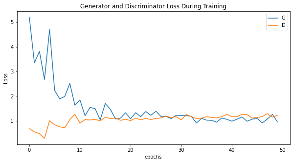
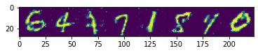
View the result, if you run the code correctly after the training is finished then we can see the loss plot and some generated result by running the code snippet bellow plt.figure(figsize=(10,5)) plt.title("Generator and Discriminator Loss During Training") plt.plot(G_losses,label="G") plt.plot(D_losses,label="D") plt.xlabel("epochs") plt.ylabel("Loss") plt.legend() plt.show() view_result(generator_model,batch=8) the plot and generated image should look like This